

Imagine a machine learning model trying to learn the secrets of a complex dataset. It’s like a detective piecing together clues but with numbers and algorithms instead of fingerprints and witness statements. In this detective work, two critical factors come into play: bias and variance.
Bias is like a pre-existing prejudice. It’s the tendency of the model to consistently favor certain patterns or make systematic errors, regardless of the data it sees. Think of it as the detective always assuming the suspect with the red shoes is guilty.
Variance is like impulsiveness. It’s the model’s sensitivity to the specific training data it receives. Imagine the detective jumping to conclusions based on a single witness account, without considering other evidence. A high-variance model might perfectly fit the training data, but stumble when faced with new, unseen examples.
The bias vs variance tradeoff is the fundamental balancing act in machine learning. It’s the delicate dance between a model’s ability to capture the underlying patterns in the data (low bias) and its ability to generalize well to new data (low variance).
So, why is understanding this trade-off so important?
- It helps diagnose model performance: Analyzing bias and variance allows us to pinpoint the source of errors, whether the model is stubbornly overfitting or blindly underfitting.
- It guides model selection and tuning: Knowing the trade-off empowers us to choose the right model for the task at hand and adjust its parameters to achieve the optimal balance between bias and variance.
- It prevents over-optimism: Understanding the limitations of our models prevents us from drawing unwarranted conclusions based on training data alone.
Mastering the bias-variance trade-off is an essential skill for any aspiring machine learning practitioner. In this tutorial, you will learn about Bias vs Variance Tradeoff.
Table of Contents
Bias and Variance in Machine Learning
In the intricate world of machine learning, accurate predictions are the holy grail. Yet, two persistent foes stand in the way: bias and variance. Understanding these concepts is crucial for developing high-performing models that navigate the delicate balance between oversimplification and overfitting.
Bias
Imagine your model consistently underestimates house prices by 10%. This systematic error, inherent to the model itself, is bias. It arises from simplifying assumptions or choosing the wrong algorithm. A straight line might perfectly fit a small set of data points, but miss the curvature of the actual housing market, leading to biased predictions.
- Bias is the difference between the average prediction of a model and the true value of the output variable.
- Bias measures how well a model can capture the true relationship between the input and output variables.
- A high bias model makes strong assumptions about the data and tends to oversimplify the problem, resulting in underfitting.
- A low bias model makes fewer assumptions about the data and tends to fit the data more closely, resulting in better accuracy.
The bias of a model can be mathematically defined as:

where ŷ is the predicted value, y is the true value, and E is the expected value operator.
Variance
Now picture a skittish model that fluctuates wildly depending on the training data. A slight change in data points could lead to drastically different predictions, like valuing the same house at $100,000 one day and $1 million the next. This sensitivity to training data variations is variance. A complex model trying to fit every data point, including noise, becomes overfitted and loses its ability to generalize to unseen data.
- Variance is the variability of the model’s predictions for different training sets.
- Variance measures how sensitive a model is to the variations in the data.
- A high variance model learns too much from the specific features of the training data and tends to overfit the data, resulting in poor generalization.
- A low variance model learns less from the specific features of the training data and tends to be more robust to new data, resulting in better generalization.
- The variance of a model can be mathematically defined as:

where ŷ is the predicted value, and E is the expected value operator.
Relationship between Bias and Variance
Bias and variance are inversely related, meaning that as one increases, the other decreases. This is because a model that fits the data more closely will have lower bias but higher variance, and vice versa. The goal of machine learning is to find a balance between bias and variance that minimizes the total error of the model.
The total error of a model can be decomposed into three components: bias, variance, and irreducible error. Irreducible error is an error that cannot be reduced by any model, as it is caused by the inherent noise or randomness in the data. The formula for the total error is:

The bias-variance trade-off is the challenge of finding a model that has low bias and low variance, and thus low total error. A common way to visualize the trade-off is by using a bullseye diagram, as shown below:
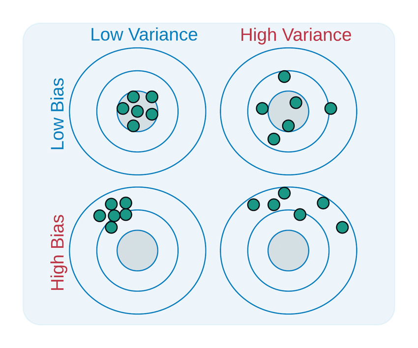
The center of the target represents the true value of the output variable, and the arrows represent the predictions of different models trained on different subsets of the data. The bias of a model is the distance between the center of the target and the average of the predictions, and the variance of a model is the spread of the predictions around their average.
As we can see from the diagram, a model with high bias and low variance makes consistent but inaccurate predictions, a model with low bias and high variance makes inconsistent but accurate on average predictions, and a model with low bias and low variance makes consistent and accurate predictions.
Effect of Bias and Variance on Model Performance
Bias and variance affect the performance of a model in terms of its accuracy and generalization ability. Accuracy is the measure of how close the model’s predictions are to the actual values, and generalization is the measure of how well the model performs on new or unseen data.
- High Bias, Low Variance: Imagine a model predicting all house prices as the average. While consistent (low variance), its predictions are far from reality (high bias), leading to poor performance. This scenario, called underfitting, happens when the model fails to capture the underlying patterns in the data.
- Low Bias, High Variance: A model trying to fit every data point like a chameleon might have accurate predictions on the training data, but its performance plummets on unseen data (high variance). This, known as overfitting, makes the model unreliable for real-world applications.
- The Sweet Spot: Ideally, we seek a model with low bias and low variance. This golden path ensures accurate predictions both on the training data and unseen data, leading to optimal performance.
The Bias vs Variance Tradeoff
In machine learning, we want to create models that can make accurate and generalizable predictions based on data. However, many factors can affect the performance of a model, such as the complexity of the data, the choice of the model, and the amount of training data. One of the most important challenges in machine learning is to find a balance between model complexity and predictive accuracy, which is known as the bias-variance trade-off.
Model Complexity and Predictive Accuracy
Model complexity refers to the number of parameters, features, or interactions that a model can use to fit the data. A more complex model can capture more details and nuances of the data, but it also requires more data and computational resources to train and test. A less complex model can be simpler and faster to train and test, but it may not be able to capture the true relationship between the input and output variables.
Predictive accuracy refers to the ability of a model to make correct predictions on new or unseen data. A more accurate model can generalize well to different data sets and scenarios, but it may also be prone to overfitting the data. A less accurate model can avoid overfitting the data, but it may also be prone to underfitting the data.
The bias-variance trade-off is the trade-off between model complexity and predictive accuracy. A more complex model can have a lower bias but higher variance, and a less complex model can have a higher bias but lower variance. The goal of machine learning is to find a model that has low bias and low variance, and thus high predictive accuracy.
The bias-variance trade-off arises because these two components of error move in opposite directions with model complexity.
- Simple models: Fewer parameters lead to lower variance but higher bias. These models are easy to train and interpret but lack the flexibility to capture complex relationships, resulting in underfitting and poor generalization.
- Complex models: Increasing the number of parameters reduces bias, allowing the model to fit the training data more closely. However, this flexibility comes at the cost of high variance, making the model susceptible to noise and prone to overfitting.
Impact of High or Low Bias and Variance on Model Performance
High or low values of bias and variance can have different impacts on the model performance, as shown below:
- High Bias:
- Accuracy on training data: High
- Accuracy on unseen data: Low
- Generalization: Poor
- Example: A linear regression model predicting house prices might consistently underestimate values, failing to capture nuanced features.
- Low Bias:
- Accuracy on training data: Low
- Accuracy on unseen data: High
- Generalization: Good
- Example: A complex neural network might perfectly fit the training data, capturing every quirk, but struggle to perform well on new, unseen houses.
- High Variance:
- Accuracy on training data: High
- Accuracy on unseen data: Low
- Generalization: Poor
- Example: A decision tree model sensitive to minor data changes might predict wildly different prices for similar houses.
- Low Variance:
- Accuracy on training data: Low
- Accuracy on unseen data: Low
- Generalization: Poor
- Example: A simple model like predicting an average price for all houses would perform poorly on both training and unseen data.
- High bias and low variance: A model with high bias and low variance can have low predictive accuracy and low generalization, as it will fail to capture the complexity of the data and make systematic errors. This is also known as underfitting the data, as the model is too simple for the data.
- Low bias and high variance: A model with low bias and high variance can have high predictive accuracy on the training data but low generalization on the test data, as it will learn too much from the specific features of the training data and make random errors. This is also known as overfitting the data, as the model is too complex for the data.
- Low bias and low variance: A model with low bias and low variance can have high predictive accuracy and high generalization, as it will fit the data well and make minimal errors. This is the ideal scenario for machine learning, as the model is neither too simple nor too complex for the data.
Navigating the Trade-Off:
Finding the optimal balance between bias and variance is crucial for building robust and generalizable models. Techniques like regularization and cross-validation can help mitigate the effects of both, leading to models that accurately learn from the data while avoiding overfitting or underfitting.
Remember, the bias-variance trade-off is a constant consideration in machine learning, and understanding its implications is key to building models that truly perform in the real world.
Balancing Bias and Variance
In machine learning, we want to create models that can make accurate and generalizable predictions based on data. However, finding a balance between bias and variance, which are two important components of the total error of a model, is not easy. A model with high bias and low variance can underfit the data, and a model with low bias and high variance can overfit the data. Both scenarios can lead to poor performance and low predictive accuracy. Therefore, we need to use techniques that can help us balance bias and variance, such as regularization, ensemble methods, and model selection.
Regularization
- Regularization is a technique that adds a penalty term to the loss function of a model, which reduces the complexity of the model and prevents overfitting.
- Regularization can be applied to different types of models, such as linear regression, logistic regression, neural networks, etc.
- Regularization can be of different forms, such as L1 regularization, L2 regularization, dropout, etc.
- L1 regularization adds the absolute value of the model parameters to the loss function, which results in sparse solutions and feature selection.
- L2 regularization adds the square of the model parameters to the loss function, which results in shrinkage of the parameters and smooth solutions.
- Dropout is a technique that randomly drops out some units or connections in a neural network during training, which reduces the co-dependence of the units and improves generalization.
- Regularization can reduce the variance of a model by introducing some bias, which can improve the trade-off between bias and variance.
Ensemble Methods
- Ensemble methods are techniques that combine multiple models to create a more powerful and robust model, which can improve the predictive accuracy and generalization of the model.
- Ensemble methods can be of different types, such as bagging, boosting, stacking, etc.
- Bagging is a technique that creates multiple models by sampling the data with replacement, and then averages or votes the predictions of the models, which reduces the variance and improves the stability of the model.
- Boosting is a technique that creates multiple models by sequentially adding new models that correct the errors of the previous models, and then assigns weights to the predictions of the models, which reduces the bias and improves the accuracy of the model.
- Stacking is a technique that creates multiple models by using different algorithms or parameters, and then trains a meta-model that learns how to combine the predictions of the models, which can capture the strengths of different models and improve the performance of the model.
- Ensemble methods can balance bias and variance by exploiting the diversity and complementarity of multiple models.
Model Selection
- Model selection is a technique that involves choosing the best model among a set of candidate models, based on some criteria or metrics, such as accuracy, error, complexity, etc.
- Model selection can be done by using different methods, such as train-test split, cross-validation, grid search, random search, etc.
- Train-test split is a method that splits the data into two subsets, one for training and one for testing, and then evaluates the performance of the model on the test set, which can provide a simple and fast estimate of the model’s generalization ability.
- Cross-validation is a method that splits the data into multiple subsets, and then uses some of them for training and some of them for testing, and then averages the results, which can provide a more reliable and robust estimate of the model’s generalization ability.
- Grid search is a method that performs an exhaustive search over a predefined grid of model parameters and then selects the best combination of parameters that maximizes the performance of the model, which can provide a fine-tuned and optimized model.
- Random search is a method that performs a random search over a predefined range of model parameters and then selects the best combination of parameters that maximizes the performance of the model, which can provide a faster and more efficient model.
- Model selection can balance bias and variance by finding the optimal model that minimizes the total error and maximizes the predictive accuracy.
Importance of Finding the Right Balance
Finding the right balance between bias and variance is important for machine learning, as it can affect the performance and quality of the model. A model that has high bias and low variance can underfit the data, which means that it cannot capture the true relationship between the input and output variables, and thus makes systematic errors.
A model that has low bias and high variance can overfit the data, which means that it learns too much from the specific features of the training data, and thus makes random errors. Both scenarios can lead to poor performance and low predictive accuracy, as the model cannot generalize well to new or unseen data.
Therefore, we need to find a balance between bias and variance that minimizes the total error and maximizes the predictive accuracy, which can result in a more powerful and robust model.
Bias vs Variance TradeOff in Action
The delicate dance between bias and variance plays out across various machine learning algorithms, shaping their strengths and weaknesses. Let’s explore some real-world examples:
1. Linear Regression vs. Decision Trees:
- Linear Regression: With its simple, linear model, it suffers from high bias when dealing with complex relationships. It might consistently underestimate housing prices, failing to capture non-linear factors like location or amenities.
- Decision Trees: Their branching structure allows for flexibility, but can lead to high variance if not carefully controlled. A deep tree might perfectly fit the training data, including noise, but struggle to generalize to unseen houses, potentially predicting wildly different prices for similar properties.
Challenges:
- Linear Regression: Selecting appropriate features and transformations to reduce bias while keeping the model interpretable.
- Decision Trees: Pruning the tree to avoid overfitting and controlling depth to prevent high variance.
Strategies:
- Linear Regression: Feature engineering, regularization techniques like L2 penalty, and incorporating interaction terms for non-linear relationships.
- Decision Trees: Setting a maximum depth, using early stopping, and ensemble methods like Random Forests to average out individual biases and reduce variance.
2. Spam Detection:
- Naive Bayes: This probabilistic classifier relies on simple assumptions, potentially leading to high bias if the true relationships between features and spam are more complex.
- Support Vector Machines (SVMs): Their ability to find optimal separating hyperplanes can result in high variance, especially with noisy data, leading to misclassifications on unseen emails.
Challenges:
- Naive Bayes: Addressing irrelevant or missing features and adapting to complex spam patterns.
- SVMs: Choosing the right kernel and parameter tuning to avoid overfitting noisy data.
Strategies:
- Naive Bayes: Feature selection and smoothing techniques to handle noisy data.
- SVMs: Regularization techniques like L1 penalty and carefully selecting kernel functions and hyperparameters.
3. Image Recognition:
- K-Nearest Neighbors (KNN): This simple algorithm, while effective with small datasets, can suffer from high variance in high-dimensional image data, leading to misclassifications due to noise or outliers.
- Convolutional Neural Networks (CNNs): Their powerful feature extraction capabilities can lead to high variance if not carefully regularized, potentially overfitting to specific training images and failing to generalize to new scenes.
Challenges:
- KNN: Choosing the optimal K value and addressing the “curse of dimensionality” in high-dimensional data.
- CNN: Regularization techniques like dropout, data augmentation, and early stopping to prevent overfitting.
Strategies:
- KNN: Dimensionality reduction techniques and outlier removal to improve performance.
- CNN: Regularization techniques, data augmentation, and ensemble methods like bagging to improve robustness and generalization.
Conclusion
Bias and Variance are two important concepts in machine learning that measure the accuracy and generalization ability of a model. They are related to the trade-off between underfitting and overfitting, which are common problems in machine learning.
The goal of machine learning is to find a balance between bias and variance that minimizes the total error of the model.
To achieve this, we can use techniques such as regularization, ensemble methods, and model selection, which can help us optimize the model complexity and predictive accuracy. By finding the right balance between bias and variance, we can create more powerful and robust models that can make accurate and generalizable predictions based on data.
Frequently Asked Questions
What is the difference between bias and variance in machine learning?
Bias is the difference between the average prediction of a model and the true value of the output variable, while variance is the variability of the model’s predictions for different training sets.
How do you reduce bias and variance in machine learning?
To reduce bias and variance in machine learning, we can use techniques such as regularization, ensemble methods, and model selection, which can help us optimize the model complexity and predictive accuracy.
What causes high bias and high variance in machine learning?
High bias is caused by using a too simple or linear model that cannot capture the complexity of the data, while high variance is caused by using a too complex or nonlinear model that learns too much from the specific features of the data.
How does the bias vs variance tradeoff affect the performance of machine learning models?
The bias-variance tradeoff affects the performance of machine learning models by balancing the model’s ability to minimize bias and variance, which is referred to as the tradeoff between model complexity and predictive accuracy.
What are the strategies for managing the trade-off between bias and variance in machine learning?
Strategies for managing the trade-off between bias and variance in machine learning include techniques for balancing both, such as regularization, ensemble methods, and model selection.